Calculus I • Math 1210

At Utah State University, Calculus I covers limits, differentiation, and integration. This page is a summary of most topics covered in Calculus I. This is a general reference guide for Calculus I topics.  This is a list that summarizes derivative, integration and identity rules.

---

Limits

Intro to limits

Limits are crucial to essentially every Calculus concept. They describe the behavior of a function near (but not at) a specified value. Two ways that this can be useful are

1. Determining behavior of a function near a point where the function isn't defined such as \(\displaystyle\lim_{x\rightarrow4}\frac{x(x-4)}{x-4}\). Although we can't directly evaluate this function at \(x=4\), we can find the limit at \(x=4\) to be 4.
2. Determining the value of a function as the input goes to infinity. \(f(\infty)\) is mathematically nonsensical, but \(\displaystyle\lim_{x\rightarrow\infty}f(x)\) is great, and means what you probably expected \(f(\infty)\) to mean.

Rules of limits

• The limit of a sum is the sum of a limit. \[\displaystyle \lim_{x \to a} (f(x) + g(x)) = \lim_{x \to a} f(x) + \lim_{x \to a} g(x)\]
• The limit of a difference is the difference of a limit. \[ \displaystyle \lim_{x \to a} (f(x) - g(x)) = \lim_{x \to a} f(x) - \lim_{x \to a} g(x)\]
• The limit of a product is the product of a limit. \[ \displaystyle \lim_{x \to a} f(x)g(x) = \Big(\lim_{x \to a} f(x)\Big)\Big(\lim_{x \to a} g(x)\Big)\]

Limits of Rational Functions

A rational function is the ratio of two polynomials, or in other words, a fraction of two polynomials. For example:
\[ \displaystyle y = \frac{f(x)}{g(x)} = \frac{\text{a polynomial}}{\text{a polynomial}}\]

Limit approaching infinity

If we take the limit of the following equation:

$\underset{x\to \infty }{lim}\frac{f(x)}{g(x)}$

where $f(x)$ and $g(x)$ are both polynomials, we can look at the orders (the highest exponents) of the two polynomials. There are three rules:

1. If $f(x)$ is higher order than $g(x)$ , then the limit is either positive or negative infinity. $\left|\underset{x\to \infty }{lim}\frac{f(x)}{g(x)}\right|=\infty$ . To decide whether it is plus or minus infinity, take the sign of the leading coefficient of $f(x)$ .
2. If the denominator is higher order, the limit is equal to zero.
3. If $f(x)$ is equal order than $g(x)$ , then the limit is the quotient of the leading coefficients: \(\displaystyle\lim_{x\rightarrow\infty}\frac{f(x)}{g(x)} = \frac{f_{\text{leading coefficient}}}{g_{\text{leading coefficient}}}\). The leading coefficient is the number multiplying the $x$ with the highest power.

Other limits

If we are taking the limit of $\underset{x\to a}{lim}\frac{f(x)}{g(x)}$   (where our numerator and denominator respectively are continuous polynomials), and $-\infty <a<\infty$ , the first thing we should try is to evaluate $\frac{f(a)}{g(a)}$ . There are three cases:

1. Case 1: $\frac{f(a)}{g(a)}=L,L\in ℝ$ . If evaluating the function yields a value, that value is the limit.
2. Case 2: $\frac{f(a)}{g(a)}=\frac{b}{0},b\in ℝ$ . If this is the case, the limit may not exist, and if it does exist, it will be $\pm \infty$ . In order to determine if our limit exists, we should evaluate the limit from the right and left separately (Both should evaluate to \(\pm\infty\)).
   
   1. If both limits have the same sign, they are both equal to your limit.
   2. If the signs are opposite, (ie; the left limit is \(-\infty\) but the right is \(\infty\)) then the limit does not exist and can only be expressed from the left or right. 
3. Case 3: $\frac{f(a)}{g(a)}=\frac{0}{0}$ . This case is of the most interest to us, since we know that $a$ must be a root of both $f(x)$ and $g(x)$ . If this is the case, we can simplify the expression until we either get a limit, or we find that one does not exist. To do this:
   1. Factor both the numerator and denominator. You should see one or more common factors.
   2. Eliminate these common factors.
   3. Re-evaluate the function according to cases 1 and 2.

The limit of \(\displaystyle\frac{\sin x}{x}\) and the "squeeze theorem"

If we are given \(\displaystyle\lim_{x\rightarrow \infty}\frac{\sin x}{x}\), this is a special case of limiting, as it's difficult to (directly) compute. However, we can use the "squeeze theorem" to evaluate this limit quite easily.

Squeeze Theorem: If $g(x)\ge f(x)$ , $\underset{x\to \infty }{lim}g(x)=a$ , $h(x)\le f(x)$ and $\underset{x\to \infty }{lim}h(x)=a$ , then $\underset{x\to \infty }{lim}f(x)=a$ .

To find \(\displaystyle\lim_{x\rightarrow\infty}\frac{\sin x}{x}\) we can start with the fact that for any \(x\), \(-1\le\sin x \le 1\). We can multiply all portions of this inequality by \(\frac{1}{x}\) and find for positive values of \(x\), \(\frac{-1}{x} \le \frac{\sin x}{x} \le \frac{1}{x}\). This inequality squeezes the function we want to take the limit of, \(\frac{\sin x}{x}\), between \(\pm \frac{1}{x}\). Because \(\displaystyle\lim_{x\rightarrow \infty}\pm\frac{1}{x}=0\), we can conclude using the squeezing that we did earlier \(\displaystyle 0\le \lim_{x\rightarrow \infty} \frac{\sin x}{x} \le 0\), and the only way that is possible, is if \(x=0\). 

Video

Here's a video working through a few practice problems involving limits.

---

Derivatives

Derivatives tell us the slope of a graph at a particular point. More specifically, derivatives tell us the slope of the tangent line at a particular point, since a function's slope can change as we traverse the horizontal axis. So, how do we get this slope at some point $(x,f(x))$ ? Well, we can approximate it by using a secant line, taking two points, $(x,f(x))$ and $(x+h,f(x+h))$ . Notice how to get the second point, we just add a distance of $h$ to the first point. The slope between these two points is $\frac{y_1-y_0}{x_1-x_0}$ , or in our case, $\frac{f(x+h)-f(x)}{x+h-x}$ , which simplifies to $\frac{f(x+h)-f(x)}{h}$ .

To get a tangent line, all we have to do is reduce $h\to 0$ . So, the slope of our tangent line then becomes $\underset{h\to 0}{lim}\frac{f(x+h)-f(x)}{h}$ . This is what is called the limit definition of a derivative. There are a lot of shortcuts you can use to compute this extremely quickly, but you must understand why it works. 

Derivative Rules

The following rules can be used to take derivatives quickly:

• Power Rule: \( \displaystyle\frac{d}{d x}\left[x^{n}\right]=n x^{n-1}\)
• Constant Coefficient Rule (Linearity): \( \displaystyle\frac{d}{d x}[a f(x)]=a \frac{d}{d x}[f(x)]\)
• Constant Rule: \( \displaystyle\frac{d}{d x}[a]=0\)
• Sum/Difference Rule (Linearity): \( \displaystyle\frac{d}{d x}[f(x) \pm g(x)]=f^{\prime}(x) \pm g^{\prime}(x)\)
• Product Rule: \( \displaystyle\frac{d}{d x}[f(x) g(x)]=f^{\prime}(x) g(x)+f(x) g^{\prime}(x)\)
• Quotient Rule: \( \displaystyle\frac{d}{d x}\left[\frac{f(x)}{g(x)}\right]=\frac{g(x) f^{\prime}(x)-g^{\prime}(x) f(x)}{g(x)^{2}}\)
• Chain Rule: \( \displaystyle \frac{d}{d x}[f(g(x))]=g^{\prime}(x) f^{\prime}(g(x))\)

---

Riemann Sums

Riemann sums are the precursor to integration, and a way to approximate the area under a curve. We have a curve, enclosed by a function, $f(x)$ , with $x\in a,b$ . To find the area, we can approximate using rectangles. To start, we choose how many rectangles to divide our domain into. Then, we sample the function at that many points. Finally, we sum up the area of each rectangle to get an approximation.

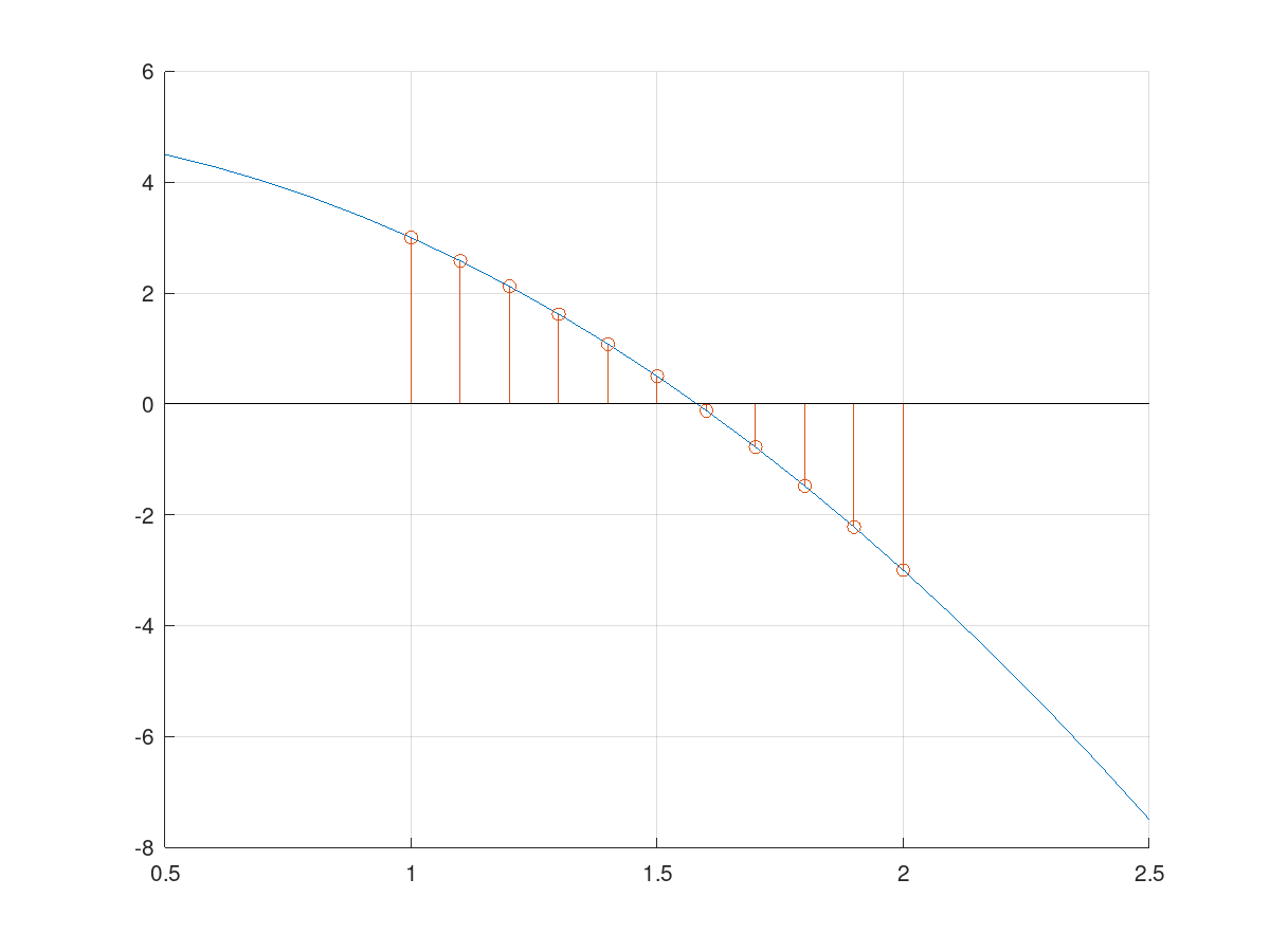
Now, in order to create rectangles for use in approximation, we can either use the sample on the left hand side of the rectangle, or the one on the right. Other variations of this approximation can include trapezoids or parabolas. Note how both left and right approximations either over-approximate or under-approximate the function, depending on the nature of the function. In our example, the left-hand approximation over estimates, whereas the right-hand approximation under estimates the area.

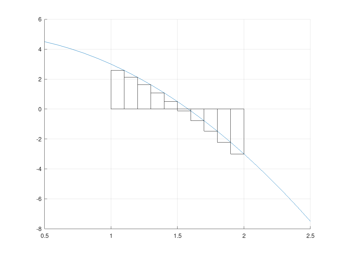
So how do we mathematically represent this? To use $n$ rectangles, we have to create a summation, either ${\sum }_{i=0}^{n-1}$ or ${\sum }_{i=1}^n$ (depending on whether we want a left-hand or a right-hand approximation), and then place the width and height of the function in that summation. The width (called $\Delta x$ ) is the same for each rectangle, just the size of the domain divided by the number of rectangles we're using; i.e., $\Delta x=\frac{b-a}{n}$ . The height is just $f(x_i)$ , with $x_i$ being the $x$ value of the $i^{th}$ rectangle. So, we evaluate $f(x)$ at $x_i$ , with $x_i=a+\Delta xi=a+i\left(\frac{b-a}{n}\right)$ (take a minute to convince yourself why that is equal to the $x$ value at the $i^{th}$ rectangle).

So, for a left-hand Riemann sum of $f(x)$ with $x\in a,b$ using $n$ rectangles, our formula looks like this:

${\sum }_{i=0}^{n-1}\Delta xf(x_i)={\sum }_{i=0}^{n-1}\Delta xf(a+i\Delta x)={\sum }_{i=0}^{n-1}\left(\frac{b-a}{n}\right)f(a+i\left(\frac{b-a}{n}\right))$

For a right-hand Riemann sum, all we have do to is change the lower and upper bound of the iterator:

${\sum }_{i=1}^n\Delta xf(x_i)={\sum }_{i=1}^n\Delta xf(a+i\Delta x)={\sum }_{i=1}^n\left(\frac{b-a}{n}\right)f(a+i\left(\frac{b-a}{n}\right))$

${\int }_a^{b}f(x)dx=\underset{n\to \infty }{lim}{\sum }_{i=0}^{\mathrm{n\; -\; 1}}(\left(\frac{b-a}{n}\right)i+a)f(\left(\frac{b-a}{n}\right)i+a)$

---

Integrals

We know the more subdivisions a Riemann sum uses, the more exact the approximation of the area under the function is. We can use a limit to take a Riemann sum as the number of subdivisions approaches infinity to find an estimation with diminishing error. In less formal words, a Riemann sum with infinite subdivisions gives us an exact answer for the area under a function. This infinite Riemann sum is called an integral and is an incredibly powerful tool.

The Fundamental Theorem of Calculus

The Fundamental Theorem of Calculus, as the name implies, is quite important. We typically write it as two theorems. The first one tells us that the integral is the anti-derivative, or in other words, integrating a function, and then taking the derivative will result in the original function. We write this theorem as
$$\frac{d}{dx}\int_a^x f(x)dx=f(x).$$ The second part of the Fundamental Theorem of Calculus says that because integrals are anti-derivatives, we can calculate definite integrals (the area under a curve) using an anti-derivative instead of a Riemann sum. This is convienient because adding up infinite rectangles is impractical or impossible when compared to finding the anti-derivative of a function. We write this part of the theorem as $$\int_a^bf(x)dx = F(b)-F(a),$$ where \(\displaystyle F(x)=\int f(x)dx\).

Integration rules

• Power Rule: $\int x^{n}dx=\frac{1}{n+1}{x}^{n+1}+C$
• Constant Coefficient Rule (Linearity): $\int af(x)dx=a\int f(x)dx=aF(x)+C$
• Sum/Difference Rule (Linearity): $\int f(x)\pm g(x)dx=\int f(x)dx\pm \int g(x)dx$

Integration techniques

$u$ -Substitution

Let's say we find an integration of the form:

$\int ag(f(x))f^{\prime }(x)dx$

This looks a lot like the chain rule ( $\frac{d}{dx}\left[g(f(x))\right]=g^{\prime }(f(x))f^{\prime }(x)$ ), right? We know from the fundamental theorem of calculus that if we integrate both sides of that chain rule, we get $g(f(x))+C=\int g^{\prime }(f(x))f^{\prime }(x)dx$ . Therefore:

$\int ag(f(x))f^{\prime }(x)dx=G(f(x))+C$

We call this $u$ -substitution, because we generally notate this as $u=f(x),du=f^{\prime }(x)dx$ . This change of variables allows us to view the integration now as:

$\int ag(u)du$

Integration by Parts

Integration by parts is based on the product rule, $\frac{d}{dx}\left[u(x)v(x)\right]=u^{\prime }(x)v(x)+u(x)v^{\prime }(x)$ . If we integrate both sides, we get:

$\int \frac{d}{dx}\left[u(x)v(x)\right]dx=\int (u^{\prime }(x)v(x)+u(x)v^{\prime }(x))dx$

$u(x)v(x)=\int (u^{\prime }(x)v(x)+u(x)v^{\prime }(x))dx$

$u(x)v(x)=\int u^{\prime }(x)v(x)dx+\int u(x)v^{\prime }(x)dx$

$\int u(x)v^{\prime }(x)dx=u(x)v(x)-\int u^{\prime }(x)v(x)dx$

Or, as it's more commonly written:

$\int udv=uv-\int vdu$

To use integration by parts, divide your integral into a u and a dv part. Make sure everything in the original integral is present in either u or dv. Next find du, the derivative of u, and v, the integral of dv. Finally, use the formula above to rewrite the original integral. If the new integral does not look simpler than, or at most equally complicated to the original integral, you might consider changing how you defined u and dv. You also may need to use integration by parts multiple times to solve the same problem.