First Order Differential Equations
Return to the Math 2250 Overview Page.
Homogeneous Differential Equations
Let's look at the most basic differential equation, a first order homogeneous differential equation. \[y' - a y = 0\] \[y(0)=A\] This equation can be rewritten so it can be solved visually as \(y'=a y\). This states that the derivative of a function is equal to the original function multiplied by some constant. If you remember from calculus, there is one primary function that can solve for this equation. That function is an exponential function. Notice as well that an arbitrary initial value was included. This information is needed to create a full solution.
The general solution to the differential equation becomes \[y(t)=Ce^{at}\]
We can now solve for the complete solution to the function \(y(t)\) by evaluating at \(y(0)=A\). The complete solution then becomes \[y(t)=A e^{at}\]We can now check our solution against the original differential equation to verify that it is a solution.\[y'(t)=A a e^{at}\]\[A a e^{at} - a(A e^{at})=0\]\[0=0\]
Example Problem Homogeneous Solution
A common problem you may encounter is a compounding interest rate problem such as the following:
You find a potential investment account that has an annual compounding interest rate of 8\%. If you put \$500 into the account to start, how much money would you have in your account after 10 years?
Given terms:\[rate = a = 0.08\]\[y(0)=\$500\]
Set up the differential equation:\[y'-0.08y=0\]\[y'=0.08y\]
Substitute our general solution:\[y(t)=Ce^{0.08t}\]
Solve for our unknown coefficients:\[\$500 = Ce^0\]\[\$500=C\]
Evaluate at \(t=10\)\[y(10)=\$500e^{0.08(10)}=\$1112.77\]
It is also a good idea to check the solution against the original differential equation to verify that it satisfies the condition.
Non-Homogeneous Differential Equations
There are five general forcing functions for differential equations that we regularly solve for. These functions include:
- Constant Forcing \(f(t)=C\)
- Exponential Forcing Function \(f(t)=A e^{ct}\)
- Sinusoidal Forcing Function \(f(t)=A \cos(\omega t),f(t)=B \sin(\omega t)\)
- Step Function \(f(t)=H(t-\tau)\)
- Delta Function \(f(t)=\delta (t-\tau)\)
When forcing terms are added to differential equations, the method to solve becomes slightly more involved. Now our solution will be determined in two parts. The first is known as the null solution. This solution is found when the forcing term is set equal to zero. This solution is equal to the homogeneous solution.
\[y'-ay=f(t)=0\]\[y_{null} = Ce^{at}\]
The second half of the solution is known as the particular solution. The particular solution is based on the given forcing input. A complete solution comes from the combination of the null and particular solution.
\[y_{complete}=y_{null}+y_{particular}\]
Initial conditions can be substituted into the complete solution to solve for the unknown coefficient on the null solution. For now, we will look at general solutions for the given functions. Each particular solution derived can be found using Green's Function which gives a solution to any input.
Constant Forcing Term
When the forcing function for a differential equation is a constant term (\(f(t)=q\)) then the solution takes the following form:
\[y_{particular}=\frac{q}{a}(1-e^{-at})\]
Where \(\textit{a}\) is the rate from the homogeneous or null solution and \(\textit{q}\) is the constant forcing term. The Complete solution to this differential equation will then be the following
\[y_c = y(0)e^{at} + \frac{q}{a}(1-e^{at})\]
or
\[y_c = Ce^{rt} + \frac{q}{a}\]
Exponential Forcing Term
When the forcing function is an exponential function with a different rate (\(f(t)=qe^{rt}\)) then the particular solution to the differential equation is the following:
\[y_p = \frac{q}{r-a}e^{rt}\]
The complete solution to the differential equation can be found as usual be adding the null to the particular.
\[y_c=Ce^{at} + \frac{q}{r-a}e^{rt}\]
Sinusoidal Forcing Term
Sinusoidal forcing functions (\(f(t)=A \cos(\omega t),B \sin(\omega t)\)) have particular solutions that involve both a sine and cosine term normally written as
\[y_p = M \cos(\omega t) +N \sin(\omega t)\]
To solve for \( \textit{M} \) and \( \textit{N} \), we take the derivative of the symbolic solution and create a system of equations. Consider the following example:
\[y'- a y=A \cos(\omega t) +B \sin(\omega t)\]
\[y_p = M \cos(\omega t) +N \sin(\omega t)\]
\[y'_p = -M\omega \sin(\omega t)+ N\omega \cos(\omega t)\]
Substitute into the original equation
\[-M\omega \sin(\omega t)+ N\omega \cos(\omega t) - a M \cos(\omega t) +a N \sin(\omega t) = A\cos(\omega t) +B \sin(\omega t)\]
Set up a system of equations by setting sine and cosine terms equal to each other
\[A = \omega N -a M\]
\[B = a N - \omega M\]
Solving for \( \textit{a} \) and \( \textit{b} \) gives the following expression.
\[M = -\frac{a A + \omega B}{\omega ^2 +a^2}\]
\[N = \frac{\omega A -a B}{\omega ^2 +a^2}\]
Substituting these terms into our particular and complete solutions gives the following expressions
\[y_p = -\frac{a A + \omega B}{\omega ^2 +a^2}\cos(\omega t) +\frac{\omega A -a B}{\omega ^2 +a^2}\sin(\omega t)\]
\[y_c = Ce^{at} -\frac{a A + \omega B}{\omega ^2 +a^2}\cos(\omega t) +\frac{\omega A -a B}{\omega ^2 +a^2}\sin(\omega t)\]
As this solution can be unwieldy, it is normally simpler to follow the steps to solve it practically rather than using the symbolic format.
Step and Delta Forcing Terms
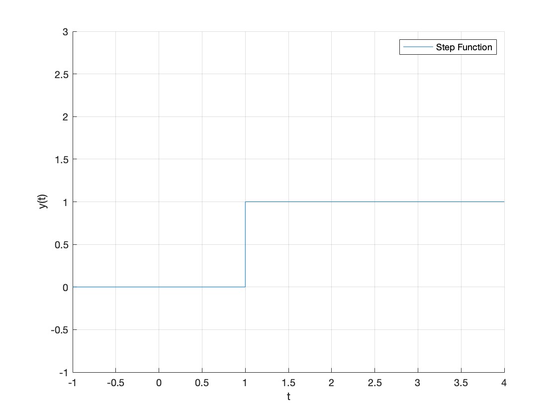
Two new functions that are introduced in differential equations are the Heaviside Step Function and the Dirac Delta Function. These functions are useful in modeling real-world engineering problems. The step function can be thought of as a light switch that gets turned on at \(t\geq\tau\). The delta function acts as a single button press or impulse of energy.Delta functions have a value of \( \infty \) at \( t = \tau \). The functions for step and delta are shown in the following figures.

The Step and Delta functions are connected functions. The delta function is the derivative of the step function.
\[\frac{d}{d t}\delta(t-\tau)=H(t-\tau)\] \[\int{H(t-\tau) d t}=\delta (t-\tau)\]
When applied to differential equations the complete solutions are the following.\[y'-a y=q(t)\]
The step function:\[y_c=y(0)e^{at}+\frac{1}{a}(e^{a(t-\tau)}-1)\]
The delta function:\[y_c=y(0)e^{at}+e^{a(t-\tau)}\]
The step function behaves like a constant forcing term but only takes effect at \(t\geq\tau\). The delta function behaves like an added null term that is added to the function at \(t=\tau\).
Solutions to Any Input
Integrating Factor
The above solutions are reliant on experience in recognizing general solutions to forcing functions. If a general solution is not known, we can solve for a complete solution to a differential equation using an integrating factor. The integrating factor allows us to simplify a first-order differential equation using the product rule and solve for a complete solution. As a review, the product rule for derivatives is:\[\frac{d}{dt}(f(t)g(t))=f'(t)g(t)+g'(t)f(t)\]
For a first-order differential equation, the integrating factor is based on the homogeneous solution. For a general differential equation (\(y'-ay=f(t)\)), the integrating factor can be solved for by:
\[\mu(t)=e^{-at}\]
This can also be used to solve for a rate that varies with time (\(a = a(t)\)). This integrating factor is written as:\[\mu(t)=e^{-\int a(t)dt}\]
To use an integrating factor to solve a differential equation, multiply it to either side and integrate the function from 0 to \( \textit{t} \).
\[\mu(t)(y'-ay)=\mu(t)q(t)\]\[e^{-at}(y'-ay)=e^{-at}q(t)\]
Decompose Left Hand Side using The Product rule\[\frac{d}{dt}(e^{-at}y)=y' e^{-at}-a y e^{-at}\]\[(e^{-at}y)\frac{d}{dt}=e^{-at}q(t)\]
Integrate both sides\[\int\limits_0^t(e^{-at}y)\frac{d}{dt}dt=\int\limits_0^te^{-at}q(t)dt\]\[e^{-at}y-y(0)=\int\limits_0^te^{-at}q(t)dt\]
Solving for \( \textit{y} \), the solution to any input using the integrating factor comes out to be\[y(t)=y(0)e^{at}+e^{at}\int\limits_0^te^{-as}q(s)ds\]
As the integration on the Right Hand Side needs to be evaluated seperately, a dummy variable of \( \textit{s} \) is used to differentiate the inside and outside terms of the integral.
Green's Function
One of the direct ways of solving for any input function is by using Green's function. As the integration can become overly complicated, it is not frequently used to solve a first-order differential equation by hand. Green's function for a first-order differential equation is written as:
\[y_p=\int\limits_o^t e^{a(t-s)}f(s)ds\]
This function naturally occurs when using integrating factor. To solve for the complete solution to a differential equation, a null term needs to be added to the particular solution as usual.
Logistic Equations
The general logistic differential equation is written as
\[y'=ry(1-\frac{y}{k})\]
These equations are non-linear equations and cannot be solved using regular methods. Two key methods include:
- Substitution \(z = \frac{1}{y}\)
- Separation of Variables
Substitution to Solve Logistic Equation
When the substitution of \(\textit{y}\) into \(z=\frac{1}{y}\) is used, the logistic equation simplifies to a first order differential equation. \[z'=-\frac{1}{y^2}y'\]
Substitute original \(\textit{y'}\)
\[z'=\frac{ry-\frac{r}{k}y^2}{-y^2}\]\[z'=\frac{r}{k}-\frac{r}{y}=\frac{r}{k}-rz\]
This gives us a general solution to our \(\textit{z(t)}\) function which. We can reintroduce our substitution to solve the logistic differential equation in terms of \( \textit{y}(t) \)
\[z(t) = Ce^{-rt}+\frac{1}{k}\]\[y(t)=\frac{1}{Ce^{-rt}+\frac{1}{k}}\]
Separation of Variables
To use separation of variables on the same generalized logistic equation, it is helpful to rewrite the Left Hand Side in different notation.\[\frac{dy}{dt}=ry(1-\frac{y}{k})\]
To separate the differential equation, we want to isolate like terms to either the left hand or right hand side of the equation. Any \(\textit{y}\) terms will be on the left while any constants or variables such as \(\textit{t}\) will be on the right.\[\frac{1}{y(1-\frac{y}{k})}\frac{dy}{dt}=r\]
We will then take the integral of both sides with respect to \(\textit{t}\)
\[\int\frac{1}{y(1-\frac{y}{k})}\frac{dy}{dt}dt=\int rdt \]
To solve the integral on the left, we will need to perform a \(\textit{partial fraction decomposition}\).
\[\frac{1}{y(1-\frac{y}{k})}=\frac{A}{y}+\frac{B}{1-\frac{y}{k}}\]\[A(1-\frac{y}{k})+By=1\]\[A=1\]\[B-\frac{A}{k}=0\]\[B=\frac{1}{k}\]
Solving the Integration on both sides becomes\[\int\frac{1}{y}\frac{dy}{dt}dt+\frac{1}{k}\int\frac{1}{1-\frac{y}{k}}\frac{dy}{dt}dt=\int rdt \]\[\ln(y)-\ln(1-\frac{y}{k})=rt + C\]
Combine Left Hand Side using Logarithm quotient rule\[\ln(\frac{y}{1-\frac{y}{k}})=rt + C\]
Evaluate every term by \( e \)\[e^{\ln(\frac{y}{1-\frac{y}{k}})}=e^{rt+C}\]
Simplify The expression\[\frac{y}{1-\frac{y}{k}}=Ce^{rt}\]\[\frac{1}{y}=Ce^{-rt}+\frac{1}{k}\]\[y(t)=\frac{1}{Ce^{-rt}+\frac{1}{k}}\]
General Solutions
First-Order Differential Equation\[y'-a y=q(t)\]First-Order Homogeneous\[y_n=Ce^{at}\]Constant Forcing Function \(q(t)=q\)\[y_p=\frac{q}{a}\]Exponential Forcing Function \(q(t)=q e^{rt}\)\[y_p=\frac{q}{r-a}e^{rt}\]Sinusoidal Forcing Function \(q(t)=A\cos(\omega t)+B\sin(\omega t)\) \[y_p=M\cos(\omega t)+N\sin(\omega t)\]\[M = -\frac{a A + \omega B}{\omega ^2 +a^2}\]\[N = \frac{\omega A -a B}{\omega ^2 +a^2}\]Delta Forcing Function \(q(t)=\delta(t-\tau)\)\[y_p=e^{a(t-\tau)}\]Step Forcing Function \(q(t)=H(t-\tau)\)\[y_p=\frac{1}{a}(e^{a(t-\tau)}-1)\]
Integrating Factor \[\mu(t)=e^{-\int a(t) d t}\]Solution to Any Input \[y_p=\int\limits_0^t e^{a(t-s)}q(s)ds\]Solution to Logistic Differential Equation \(y'=ry(1-\frac{y}{k})\)\[y(t)=\frac{1}{Ce^{-rt}+\frac{1}{k}}\]