Introduction to Statistics • Stat 1040/1045

At Utah State University, Introduction to Statistics covers conceptual understanding and statistical thinking. This page is a summary of most topics covered in Intro Statistics.

Helpful Links

Desmos Graphing Calculator

Stat 1040 Formulat Sheet | Hadfield

Stat 1040 Notes | Loveland

Normal Table for Calculating a Z-score

Fun With Stats Calculator

Use Calculator

Intro to Statistics Topics Playlist

Watch Videos

Equations

Histograms

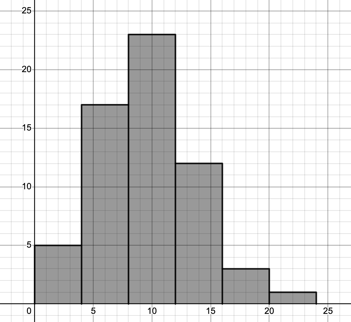
$Histogram with bins from 0 to 4, 4 to 8, 8 to 12, 12 to 16, 16 to 20, and 20 to 24. The first bin has a frequency of 5, the second a frequency of 17, the third a frequency of 23, the fourth a frequency of 12, the fifth a frequency of 5, and the sixth a frequency of 1. Altogether, this is a unimodal distribution, with a slight skew to the right side.$

$\displaystyle \text{height} = \frac{percentage}{width} $

Area Under A Normal Curve

$Standard Normal Curve pictured, with a mean of 0 and a standard deviation of 1. Between -1 and 1 lies 68% of the data. Between -2 and 2 lies 95% of the data. Between -3 and 3 lies 99.7% of the data. The data forms a bell curve, with a symmetric distribution.$

$ \displaystyle \text{Empirical Rule: } 68 - 95 - 99.7 $

$\displaystyle z = \frac{x- \text{average}}{SD}$

$\displaystyle x = \text{average} +z(SD)$

Linear Regression

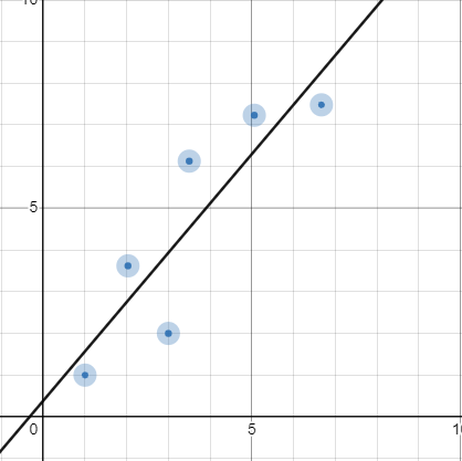
$Generic graph of linear regression line.$

$\displaystyle \text{rms error} =\left(\sqrt{1-r^{2}}\right)$ SD $\displaystyle _{Y}$

$\displaystyle \text{slope} = \frac{r(SD_Y)}{SD_X}$

$\displaystyle \text{Intercept} =\text{average}_Y - \text{slope}(\text{average} _X) $

Box Models

$Generic Box Model. 2 tickets [1] 3 tickets[0]$

$\displaystyle \mathrm{SD}_{1-0 \text { box }}=\sqrt{(\text { proportion of } 1\mathrm{~s}) \times(\text { proportion of } 0\mathrm{~s})}$

$\displaystyle \mathrm{EV}_{\text {sum }}=\text{( number of draws)} \times \text{(average of the box)} $

$\displaystyle \mathrm{SE}_{\text {sum }}=\mathrm{SD}_{\text {box }} \times \sqrt{\text { number of draws }}$

$\displaystyle \mathrm{EV}_{\%}=\% \text{ of } 1\mathrm{~s}\text{ in the box} $

$\displaystyle \mathrm{SE}_{\%}=\frac{\sqrt{\text {number of draws}} \times \mathrm{SD}_{\text {box }}}{\text { number of draws }} \times 100 \%$ or $\displaystyle \mathrm{SE}_{\%}=\frac{\mathrm{SD}}{\sqrt{\text { # of draws }}} \times 100 \%$

$\displaystyle SE_{\text {avg }}=\frac{\sqrt{\text { number of draws }} \times S_{\text {box }}}{\text { number of draws }}$ or $\displaystyle S E_{\text {avg }}=\frac{\text { SD }}{\sqrt{\text { # of draws }}}$

Hypothesis Tests

$\displaystyle z=\frac{\text{observed}- \text{expected}}{SD}$

$\displaystyle \mathrm{SD}^{+}=\sqrt{\frac{\text { sample size }}{\text { sample size }-1}} \times \mathrm{SD}$

$\displaystyle \mathrm{SE}_{\text {diff }}=\sqrt{\left(\mathrm{SE}_{\mathrm{A}}\right)^{2}+\left(\mathrm{SE}_{\mathrm{B}}\right)^{2}}$

$\displaystyle \chi^{2}=\operatorname{sum} \text{ of }\frac{\text {(observed count - expected count)}^{2} }{\text { expected count }}$

$\displaystyle \text{Expected Count} =\frac{(\text { row total) }(\text { column total })}{(\text { table total })}$